| Compiled by A. Kaplunovsky |
|
Coventry University Programme in Israel Ruppin Institute for Higher Education, Israel, 1998 |
Exercise 1.
Consider the systems of equations involving two variables
| ||||||||||||||||
Set up a vector x of integers from -10 to 10 and draw the graph using the MATLAB routine plot(x,y). Use the MATLAB routines grid to put up some grid lines on the graph, and hold to hold the graph and not erase it when you plot a second draft. Read of the graph the solution of this system.
Exercise 2.
Enter the following matrices into MATLAB:
| |||||||||||||||||||||||||||||||||||||||||||||||||||||||||||||
In MATLAB, type
| 1+2 | 2-1 | 2*3 | 23 |
| A+A | A-A | A*A | A3 |
| A+B | A-B | A*B | C2 |
| B+A | B-A | A*C | |
| A+C | -(B-A) | C*A | |
| 1+C | A-C | 2*B | |
| 1-C |
a) Did MATLAB refuse to do any of the requested calculations? Why?
b) What did 1+C and 1-C do? Is that what you expect?
c) Does A*B = B*A in general?
Exercise 3.
Solve the linear system
| ||||||||||||||||||||||
as the matrix problem.
a) Create the augmented matrix
| |||||||||||||||||||||||||||||
Solve it using the MATLAB routine rref to reduce a matrix in one single call. Ask MATLAB show you a movie of row reduction for this matrix by typing rrefmovie(A).
b) Creating the matrix
| |||||||||||||||||||||||
and the vector
| |||||||||||
Check your solution typing x = inv(A)*b or x = A\b.
Exercise 4.
Let
| |||||||||||||||||||||||
Compute det(A) and inv(A) in MATLAB.
Compute det(A) by hand and verify the determinant calculated by MATLAB. Use MATLAB to check that inv(A) is the inverse of A by computing inv(A)*A and A*inv(A).
Exercise 5.
Find the cubic polinomial p = x3+ax2+bx+c which roots are 1, Ö2 and p. Plot p over the interval [0;4].
Exercise 6.
Find the roots of p = x4-2x3-13x2+14x+2. Plot p over the interval [-5;5].
Exercise 7.
Consider the set of parametric equations:
| ||||||||||||||||
a) Use the MATLAB routine plot to sketch the graph of the parametric equations. Label the x- and y-axes and place an appropriate title on your graph. Obtain a printout of your result.
b) Try the MATLAB routine comet for a cool ride on the curve.
Exercise 8.
Suppose that a subspace S of R4 is given as follows:
| ||||||||||||||||||||||||||||||||||||||
Let the matrix A be given by
| |||||||||||||||||||||||||||||
Let the linear transformation LA:R4® R3 be given by LAx = Ax. Find a basis for the image of S using LA (i.e. LA(S)).
Exercise 9.
The following is a basis for P5:
|
|
Exercise 10.
Use MATLAB to help you write down a basis for each of the spaces R(AT), N(A), R(A) and N(AT) if
| ||||||||||||||||||||||||||||||||||||
Use MATLAB to help verify that in this case N(A) = (R(AT))^ and N(AT) = (R(A))^.
Use MATLAB to compute a basis for S^ if
| ||||||||||||||||||||||||||||||||||||||
Exercise 11.
.Find an orthonormal basis for the subspace S of R4 spanned by
| ||||||||||||||||||||||||||||||||||
Exercise 12.
Construct a symmetric matrix A by using the following MATLAB commands:
A = round(5*rand(6))
A = A+A¢
a) Compute the coefficients of the characteristic polynomial of A by typing p=poly(A). Find the roots of the characteristic polynomial to compute the eigenvalues of A by typing r=roots(p). The vector r should contain the eigenvalues of A.
b) Type e=eig(A). Now e should contain the eigenvalues of A. Compare e and r. Do they agree?
c) Compute the following quantities
The determinant of A: det(A).
The product of the eigenvalues of A: prod(e).
The trace of A: trace(A).
The sum of the eigenvalues of A: sum(e).
Which of these quantities are equal?
Exercise 13.
Consider a matrix
| ||||||||||||||||||||||||||||||||
a) Decomposite it for P,L and U matrices by the Gaussian elimination process with row pivoting.
b) Compare your solution with the result of MATLAB command [P,L,U]=lu(A).
c) What is a difference in permutation matrices?
Exercise 1.
For the following three functions:
f1(x) = 2x2-3x+4
f2(x) = x6-5x3+8x-10
f3(x) = sin(x)
use the Taylor series with an initial point x = 1 and values of h = 0.01, 0.05, 0.1, 0.5, 1.0, 2.0. Obtain results for zero- through third-order expansions.
Exercise 2.
Write a program that will evaluate the Maclaurin series for the exponential function ex.
Check your accuracy using the built-in exponential function. Use a few different values of x for this (eg. 0, 0.5, 1, 5).
Exercise 3.
Find the integral
|
Plot the integrand and its indefinite integral on the same graph over the interval Ö2+0.1 £ x £ 2
Exercise 4.
Find the roots of p = x3-2x-5. Are all the roots real? Evaluate p at its roots. Do you get zero in each case? Explain. Plot p over the interval [-2;3].
Exercise 5.
Find the cubic polinomial p = x3+ax2+bx+c which roots are 1, Ö2 and p. Plot p over the interval [0;4].
Exercise 6.
Find the roots of p = x4-2x3-13x2+14x+2. Plot p over the interval [-5;5].
Exercise 7.
Consider the set of parametric equations:
| ||||||||||||||||
a) Use the MATLAB routine plot to sketch the graph of the parametric equations. Label the x- and y-axes and place an appropriate title on your graph. Obtain a printout of your result.
b) Try the MATLAB routine comet for a cool ride on the curve.
Exercise 8.
Consider the polar equation
|
a) Use the MATLAB routine polar to plot the graph over the interval 0 £ q £ 2p. For accuracy, take at least a thousand points.
b) Change to Cartesian coordinates using the appropriate transformations and use the MATLAB routine plot to produce a graph. Label the x- and y-axes and place an appropriate title on your graph. Obtain a printout of your result.
c) Try the MATLAB routine comet for a cool ride on the curve.
Exercise 9.
Consider the path defined parametrically by the equations
| ||||||||||||||||
a) Set up the integral defining the surface area of the resulting figure if the path is revolved about the x-axis.
b) Use the MATLAB routine quad to approximate this integral.
Exercise 10.
Consider the equation
|
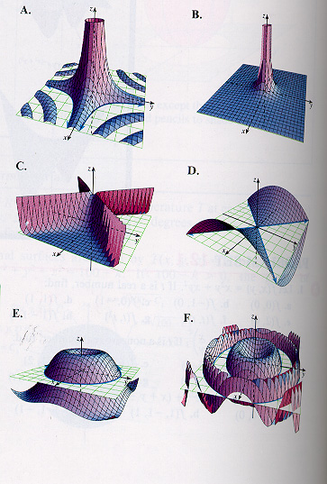
Use MATLAB to sketch the graph of the surface represented by this equation. Note: Proper advance planning will help avoid the complex number problem.
Exercise 11.
Consider the equation
|
Use Matlab to sketch the graph of the surface represented by this equation. Include the statement hidden off in your m-file to disable hidden line removal so that you can ``see through'' your image.
Exercise 12.
1. Let
| ||||||||||||
a). Is f integrable on [0,2]? Give reasons for your answer.
b). Graph f over this interval. Use the MATLAB commands
x = [0:.01:2]; y = 1./sqrt(x); y(1) = 0; plot(x,y); title('Graph of 1/sqrt(x)'); xlabel('x-axis'); ylabel('y-axis').
You can ignore the warning about division by zero. This is the reason we have explicitly redefined the first entry of y to be 0.
c). Paying no attention to the hypotheses of the Fundamental Theorem of Calculus, use it to evaluate by hand the integral from 0 to 2 of f.
d). Use MATLAB to find the Riemann sum for n = 100 in the Right Endpoint Method of this integral. Hint: The intercalation points here are
xr = [.02:.02:2] and the values of f at these points are the entries of
yr = 1./sqrt(xr) The Riemann sum is thus RSr = .02*sum(yr).
e). Use MATLAB to find the Riemann sum for n = 100 in the Left Endpoint Method of this integral. In doing this you will have a problem with division by zero. Redefine the first entry of y to be zero.
f). Use MATLAB to find the Riemann sum for n = 100 in the Midpoint Rule of this integral.
g). What is your impression now - is f integrable on [0,2] or not? Explain.
h). Find a regular partition P of [0,2] such that ||P|| < = .01, and an intercalation x*i, such that the resulting Riemann sum is larger than a million. Use Matlab to evaluate it to verify that its value is indeed larger than a million.
Exercise 13.
a). Graph Tschirnhauser's cubic equation
|
in a sufficiently large window that you see that part of the curve forms a loop. Use the script fplot('sqrt(x.2.*(x+3))',[a b]); hold; fplot('-sqrt(x.2.*(x+3))',[a b]); grid
where [a,b] is the interval over which you want x to run. (The apostrophes are needed because this is a symbolic operation). The hold command holds the first graph so that the second can be superimposed on it.
b). Use the Midpoint Rule with n = 400 to approximate the area of this loop.
c). Find the exact area. Hint: remember that on the interval [-3,0], you have sqrt(x2) = -x. Use the symmetry of the loop about the x-axis.
Exercise 14.
Consider the functions y1 = x2-x and y2 = sin(x2).
a). Graph these functions on the same set of axes to see the region that they bound. Label the axes, put an appropriate title on the graph and put a grid on the graph. Hint: decide on the appropriate domain vector x (several tries might be necessary for this) and then use plot(x,y1,x,y2).
b). From the graph you will see that these two functions meet at two points, one of which is the origin. The x-coordinate of the other point can be estimated from the graph. Suppose your estimate is denoted a. Use the MATLAB routine fzero to obtain a very good estimate for this x-coordinate. To do this, you will first have to make a function m-file for the function x2-x-sin(x2).
c). Use the Trapezoidal Rule with n = 100 to approximate the area of the region bounded by these two curves.
Exercise 15.
Consider the approximations to the integral
|
a). Graph [Ö(4-x3)] over the interval [-1, 1].
b). Use Simpson's Rule with n = 100 to approximate I. Hint: you might want to separate the odd indexed points xi from the even indexed points as follows. Let xodd = [-1+.02:.04:1-.02]; xeven = [-1+.04:.04:1-.04];
c). Find and graph the fourth derivative of f over the interval [-1,1]. Use the MATLAB symbolic differentation operator diff. The script f4 = diff('sqrt(4-x3)',4); fplot('f4',[-1 1]) returns the fourth derivative f4 and graphs it.
d). From the graph you can see where the maximum value of the absolute value |f4| occurs, say at the point x0. Find this value to obtain an upper bound K of |f4|.
e). Use K to estimate the error.
f). Use the numerical integrator quad8 to find I.
g). How does the actual error compare with the error estimate in part e)?
h). How large should n be to guarantee that the size of the error in using Simpson's Rule is less that 10-5?
Exercise 16.
Consider the integral
|
a) Verify that an antiderivative of y is F = -5e-x/5(x+5), so that the integral is equal to
|
b) Approximate this integral by Mn using the Midpoint Rule for n = 5, 10, 20, 40. Calculate the error En = |A - Mn| and see how this changes with n by calculating En/E(n+1).
Exercise 17.
Write a script which carries out Simpson's Rule for n = 6, 12, 24 and 48 to approximate
|
a) Verify that F(x) = 0.5x2(ln(x)-0.5) is an antiderivative of xln(x). Use it to calculate the value of A by hand.
b) From the MATLAB command window open a new m-file on which you will type your script. Your script should do the following:
c) Use a for-loop to: carry out Simpson's Rule to approximate the integral A from 1 to 3 of xln(x) for the cases where the number of subintervals is n = 6, 12, 24, 48;
d) Make a table whose first row consists of the values of n, whose second row consists of the values of Sn and whose third row consists of the values of the error |A - Sn|.
e) Use a for-loop to make a table of the values of the ratios of the successive errors.
Exercise 1.
Can you reproduce the following graphs using the following functions?
| |||||||||||||||||||||||
Exercise 2.
Graph the following functions and try to guess their limits.
| ||||||||||||||||||||||||||
Exercise 3.
Find the minimum of the Rosenbrock banana function:
|
Create the m-file banana.m for the function f = banana(x) as
|
Start from a point(-1.2;1) using the statement [x,out] = fmins('banana', [-1.2, 1], [0, 1.e-8], [], sqrt(2)); This statement sets the new parameter to sqrt(2) and seeks the minimum to an accuracy higher than the default.
Exercise 4.
Find the minimum of a function
|
Use the method of steepest descent, and the simplex method as implemented by the MATLAB routine fmins. Plot up the contour lines of this function on x Î [0.5;1.5] and y Î [0;2] using the MATLAB routine contour. Compare the number of iterations for both methods.
Exercise 5.
a) Sketch the graph of ¶f/¶x = 0 and ¶f/¶y = 0 in the xy-plane. Use the substitution method to find the points of intersection of these two curves. Label each point of intersection with its coordinates on your graph. Note that these points of intersection are the critical values of the function f.
b) Use MATLAB to create a sketch of the level curves of the function f
that highlight the behavior at the critical points found in part (a).
c) Use MATLAB to superimpose the gradient field of the function f on the contour plot you made in part (b). Hint: Use a grid that is coarser than that used in part (b) and scale the gradient vectors to a larger size.
d) Use the contours and gradient field developed in parts (b) and (c) to classify the extrema at each critical value. Clearly indicate this result on the printout developed in parts (b) and (c).
e) Use the second derivative test to classify extrema at each critical value found in part (a). Set up a table identical to the one used in class to summarize your results. Check that these results agree with your findings from part (d).
Exercise 6.
Integrate the function
|
where a and b are the major and minor axes of the bounding ellipse, respectively.
a) Plot up this function over its domain. Take a = 2 and b = 1. Use MATLAB function mesh for plotting this figure. Plot a countour of the bounding ellipse.
b) Consider two nested integrals. The inner integral integrates over:
|
and the outer integral integrates over -a < x < a. Use the MATLAB routine quad for the calculation of the inner integral. Write the procedure as m-file function inner. In the main program just integrate over the outer loop: integ=4*quad('inner',0,a) where the inner loop is given in the attached function inner.m, which returns the integral over y for an array of input x's.
Exercise 7.
Integrate the function f(x,y) = exy over the circle x2+y2 < 1, using Monte Carlo method.
Use the MATLAB routine rand to create random values of x and y. How many points you need for the error less then 4% for this integrand?
Exercise 8.
Consider the motion of a cannon ball which is fired straight up into the air. The initial velocity is given by U0, the mass is M, and the radius is R. We want to calculate how high the cannon ball gets, and how long it takes before it hits the ground again (e.g., how long do we have to get out of the way). The motion of the ball is governed by Newton's equations of motion, and in addition to the force of gravity we also have an air drag. This drag is given by:
F = - sign(U)*0.5*p*R2*U2*dens_air
If the mass M is 3000g, the initial velocity U0 is 2*104 cm/s, the density of air is 0.001 g/cm3, and the radius is 10cm, calculate the maximum height and the time for the ball to hit the ground again.
You can solve this problem using the shooting method. Look at the angle of elevation for a cannon necessary to hit a target. The shooting method is used to convert a boundary value problem into an initial value problem. In the case of a cannon, we are following the trajectory of the cannon ball. We know where it starts from (the location of the cannon) and its initial speed (determined by the amount of gunpowder used), but we have to figure out what angle of elevation is necessary to hit a target some distance away. Define the vector y = [x,z,vx,vz] and write down evolution equations describing their change in the attached function cannonball.m. Use a 3-stage Runge-Kutta method. Employ the MATLAB routine fzero to find the angle which yields the correct height at the required distance. To do this we must put the integration routine in a function which returns the difference between the height of the cannonball and the target at the distance of the target. We will call this function deltah(theta). The MATLAB routine fzero will adjust theta until the value returned by this function is zero.
Exercise 1.
Solve the differential equation
|
with the Euler's and Runge-Kutta methods. Use MATLAB functions ode23 and ode45 with the time step h = 1.
Exercise 2.
Use Euler method to solve the system
| ||||||||||||||
on the interval [0,15] with initial conditions
| ||||||||||||||
Do this with n=200, 400, 800, 1600, and 3200. Show that the exact solution is
| ||||||||||||||
Make a phase plot for n=200 and n=3200. Tabulate the errors and ratios of errors for this problem.
Exercise 3.
a) Find the general solution to the system x¢ = Ax, where
| ||||||||||||||||||||||||||||||||||||
b) Find the solution to the system with initial conditions x(0) = x0, where
| ||||||||||||
Exercise 4.
Consider a family of parabolas defined by
|
Find and plot a family of curves that represent the orthogonal trajectories for these parabolas (choose several values for the constant c to make the curves easy to visualize) . Show that the curves are indeed orthogonal by magnifying a portion of the plot. Do the curves intersect at right angles? Be careful with the aspect ratio of the MATLAB plots!
Exercise 5.
Use the explicit finite difference methods to compute the numerical approximation of the differential equation
| ||||||||||||||
Remember that the exact solution to this problem is:
|
Use a discretization with J = 20 so that Dx = 0.05. Use the explicit finite difference method to approximate the solution for 0 < t < 0.5. For each case given below printout the results at x10 for each time step. Plot a graph of u(x10,tn) and U10n against tn for each case.
Case 1: Use Dt = 0.00125
Case 2: Use Dt = 0.0015
Case 3: Use Dt = 0.001
Observe the difference in the results for three cases and explain the results.
Exercise 6.
Solve the harmonic oscillator problem
| ||||||||||||||||||||||||||||
by Runge-Kutta Method.
Use ode45 and plot (y1,y2),(t,y1) and (t,y2), when t0 = 0 and T = 4p with t = linspace(t0,T,300).
Exercise 7.
Examinate the predator-prey system, where the rabbit population to be given by y(1) and the fox population to be y(2). The populations vary according to the equations:
|
where a = 2, b = 1, and c = 2 are some constants describing the growth and coupling of the populations.
Use of an adaptive step size algorithm to improve the accuracy of integration. Put in more points in the region where the function curvature is large, much the same way as was the case in adaptive quadrature. Use the adaptive quadrature routine ode23.m. Set initial conditions, and decide on a tolerance. Integrate this from t = 0 to t = 15. Examine the evolution of the step size. Hint: run MATLAB demo program odedemo.
Exercise 8.
Solve the equation y"+ly = 0 with boundary conditions: y(0) = 0,y¢(1) = 0 in standard Sturm Liouville form.
Write the MATLAB routine slsolve.m which requires that you define the functions p, q, and w as well as boundary conditions in standard Sturm Liouville form. For this problem the functions p, q, and w are: p = 1; q = 0 and w = 1. The boundary conditions could be described by the array: bc = [1,0,0,1] ; n=50.
Run [lambda,eigenvec]=slsolve('pfun','qfun','wfun',bc,n) and examine the results. List the first five eigenvalues: lambda(1:5)..5/pi .Note that the eigenvalues match what we expected pretty well, except that the error is increasing as we go to higher eigenvalues. Plot the calculated eigenvalues against the exact values Examine the first five eigenfunctions : x=[0:1/n:1] and plot them.
Exercise 9.
Consider the boundary value problem defined on the interval 0 < x < [(p)/ 2] by
|
with bc: y(0) = 0, and y([(p)/ 2]) = 1.
a) Determine what choice of h will assure, a priori, that the numerical solution with the central difference method exists and is unique.
b) Using h = [(p)/ 100] and the central difference method, find the numerical solution and compare graphically your result with the exact solution y = sin(x).
Exercise 10.
Using h = 1/3, find a numerical solution of the boundary value problem defined by
|
with bc: y(0) = 0, and y(1) = 1. Be sure that the tridiagonal system which you set up has a unique solution. Compare your results with the exact solution y = x.
Exercise 11.
Consider the boundary value problem defined on the interval 0 x 6 by
|
with bc: y(0) = -1, and y(6) = 5. whose exact solution is y = x-1.
Using h = 0.5 and the upwind difference method, develop a numerical solution and compare with the exact answer.
Exercise 12.
|
with bc: y(0) = 1, and y¢(0) = 0.
Integrate from x = 0 to x = 1 with various stepsizes and compare the efficiency and accuracy with two other methods discussed. Note that you will have to use some special procedure, such as a Taylor series, to generate the value of y1 = y(h) needed to start the three-term recursion relation.
Exercise 13.
Apply interaction methods to the boundary value problem defined on the interval 0 < x < 1 by
|
with bc : y(0) = 0, and y(1) = 100.
a) Using the Jacobi method with an initial estimate of y being linear, iterate with a tolerance of 5x10⁻⁴ and h = 0.1. Be sure to count the number of interations necessary to achieve the specified accuracy at every point.
b) Modify your code to perform the Gauss-Seidel method with no over relaxation. What kind of improvement do you find over the Jacobi method?
c) Modify your code again to incorporate successive over-relaxation (SOR) with the Gauss-Seidel method. Experiment with different values of the relaxation parameter to find the value producing the fewest iterations. What kind of improvement do you find over the straight Jacobi and Gauss-Seidel methods?
Exercise 14.
Approximate the maximum eigenvalue of the boundary value problem defined by
|
with bc: y(0) = y(1) = 0, where l > 0 is a positive constant.
Exercise 15.
Consider the following mildly nonlinear boundary value problem defined on the interval 0 < x < 1 by
|
with bc: y(0) = 0, and y(1) = 0.
a) Find a numerical solution for h = 0.2 using a generalized Newton's method with w = 1.3 to solve the tridiagonal system.
b) Repeat the calculation for h = 0.1 and w = 1.3.
Exercise 16.
Using the finite element method with piecewise parabolic interpolating function P(x), approximate the minimum of the functional
|
subject to the boundary conditions y(0) = 0 and y(1) = 1. Find the exact solution of the problem and compare your numerical result with it.
Exercise 17.
Find the numerical solution of the Dirichlet problem for Laplace's equation for which
|
and g is the rectangle whose vertices are (0,0),(5,0),(5,4),(0,4)
Exercise 18.
Find the numerical solution of the Dirichlet problem for Laplace's equation for which
|
and g is the circle of unit radius whose center is (1,1)
Exercise 19.
Given the initial-boundary problem for
|
with a = 1, g1(y) = 0, g2 = e-y, f1 = x, f2 = x2, find the numerical solution at y = 5.
Exercise 20.
Here's a classic mathematical problem that goes back to Leonardo Fibonacci (? - ca 1250). To get a neat formulation, we're going to make the extreme assumptions that every pair of rabbits matures in one month, and produces a pair of baby rabbits the month after reaching maturity and every month thereafter. Start with one pair of baby rabbits at the beginning of Month 0. At the beginning of Month 1 this pair matures, but there will still be only one pair of rabbits. By the beginning of Month 2, however, there will be two pairs: the original pair, plus one new baby pair born to that original pair. By the beginning of Month 3, there will be only one more pair, for a total of three pairs, because the baby pair is not yet able to reproduce. By the beginning of Month 4, however, there will be a total of five pairs, three from the preceding month, plus two more born to the pairs that were mature that preceding month.
a) Derive a difference equation that specifies r(n), the number of rabbit pairs at month n, in terms of r(n-1) and r(n-2). Note that r(0) = 1, r(1) = 1, r(2) = 2, r(3) = 3, r(4) = 5, ...
b) Draw a block diagram of the system.
3) How many rabbit pairs will there be after one year? Write a simple MATLAB program.
4) Do you think this system is stable?
5) Can you derive a closed-form expression for r(n) that is a function of n only?
6) Find R(z), the Z transform of r(n), and then find r(n) by an inverse Z transform operation. Compute r(12), the number of rabbit pairs after 12 months, two ways: manually from the difference equation, and using your formula for r(n). Do your answers agree?
Exercise 21.
The MATLAB routine conv can be used to compute the convolution of two signals. The MATLAB routine filter also be used to compute the convolution of two signals directly. Consider the two signals
x1(n) = {0.25,0.5,1/0,0.5,0.25}
x2(n) = 2.0[u(n)-u(n-10)]
a) Use MATLAB to compute the convolution of the two given signals using conv and using filter and compare your results.
b) Plot of the convolution of the two signals using the stem plot routine.
c) Comments based upon your comparison of the two approaches to computing the required convolution.
Exercise 22.
The MATLAB routine residue can be used to perform partrial fraction expansion. Use the command ``help residue'' to see how to use this routine for partial fraction expansion of the following Z-Transform
|
a) Perform partial fraction expansion on the given H(z) divided by z rather than on H(z) itself. This makes obtaining the inverse transform easiser.
b) Use MATLAB routine freqz to obtain the frequency response of a discrete-time system.
Exercise 23.
Consider the classical problem taken from mechanical vibrations.
A mass is supported by a spring and damper and acted upon by a time-varying force. The equation of motion is:
|
where x is the displacement from the equilibrium position, m is the mass, c is the damping coefficient, k is the spring constant, F0 and w are the forcing amplitude and frequency, respectively. This equation can be recast as two first order ODE's to be solved simultaneously.
Solve this system for the time interval from 0 to 20 seconds using the following data:
m = 100 kg
c = 50 N.s / m
k = 1000 N/m
F0= 1000 N
w = 5 rad/sec
with the initial conditions x = 0 and x¢ = 0 at time t = 0.
What tests did you perform to verify your solution? For the conditions stated, how long does it take for the transient solution to die out? What is the steady-state amplitude? What are the maximum and minumum deflection and velocity?
Exercise 1.
a) Find a basis for the null space and image space (range) of
| |||||||||||||||||||||||
b) Find the eigenvalues and (possibly generalized) eigenvectors of
| ||||||||||||||||||||||||||||||||||||
c) Prove the statement that similar matrices have the same eigenvalues
d) Did you know that eigenvectors can be used to decouple quadratic equations? Find a similarity transformation, x = Py, such that the quadratic 16x12+4x1x2+9x22 = 1 has NO cross terms in y (hint: write quadratic as xTQx = 1 then choose the orthonormal eigenvectors of Q as your similarity transformation.)
e) Plot the above equation in y coordinates. Use your similarity transformation to then plot the quadratic in the original x coordinates.
Exercise 2.
a) Find the eigenvectors and eigenvalues of
| ||||||||||||||||||||||||||||||||||||
What is the degeneracy for this matrix?
b) Prove that the trace of a matrix equals the sum of its eigenvalues
c) Prove that the determinant of a matrix equals the product of its eigenvalues
d) Find the characteristic equation of
| ||||||||||||||
Denote this equation by l2+c1l1+c0l0 = 0. Calculate the matrix formed from the sum: A2+c1A1+c0A0 . Is the result surprising?
Exercise 3.
Let
| ||||||||||||||||||||||||||||||||||||||||||||||||||||||||||||||||||||||||||
a) What are the eigenvalues of A?
b) What is the degeneracy of A (both q1 and q2 )
c) Find a set of linearly independent eigenvectors (possibly generalized) of A
Exercise 4.
A is a 7x7 matrix with the folowing properties: l1 = l2 = l2 = l4 = 3 and the rank of [A-3I] = 6; l5 = l6 = l6 = -5 and the rank of [A+5I] = 5.
a) Find a Jordan Form of A.
b) If the similarity transform which puts A into Jordan form is P = [P1 P2 P3 P4 P5 P6 P7], state whether each Pi is a true-blue eigenvector or a generalized eigenvector.
Exercise 5.
Let
| ||||||||||||||
Find eAt using:
a) Cayley-Hamilton
b) PeJtP-1
c) Laplace transforms
Exercise 6.
Consider the differential equation
|
Find the time-varying state variable model if x1 = y and x2 = dy/dt
Exercise 7.
Find a state variable model for the coupled differential equation:
|
Exercise 8.
Use the Laplace Transforms to solve
|
Exercise 9.
Given the model
| |||||||||||||||||||||||||||||||||||||||||||||||||
when the input is w(t) = [d(t),u(t)]T. (Hint: try decoupling the system first using the similarity transformation, x = Pz. MATLAB could be helpful here!)
a) Identify the zero-input and zero-state solutions, then find x(t) if the initial condition is x(2) = [4-82]T and the input is w(t) = [10d(t-3),10u(t-3)]T.
b) Find the state transition matrix, F(t,t0) if
| |||||||||||||||||||||||
and verify that A(t) commutes with òA(t)dt.
Exercise 10.
Consider the system
| ||||||||||||||||||||||||||||||||||||||||||||||||||||||||||||||||||||||||||||
a) Determine the eigenvalues of the open loop system. Is the system asymptotically stable?
b) Determine if the system is controllable
c) Determine if the system is stabilizable
d) Determine whether or not Ac (i.e., the controllable part) is cyclic
e) Find w = -Kx which will set all the controllable eigenvalues to {-5}
f) What is the settling time of the closed-loop system?
Exercise 11.
Consider the system
| |||||||||||||||||||||||||||||||||||||||||||||||||||||||
a) Determine the controllable and uncontrollable eigenvalues of the system
b) Is the system stabilizable?
c) Find w = -Kx to assign all the controllable eigenvalues to {-6}. Be sure to check the eigenvalues of (A-BK)
d) What is the settling time of the closed-loop system?
Consider the system
Exercise 12.
Consider the system
| ||||||||||||||||||||||||||||||||||||||||||||||||||||||||||||||||||||||||||||
a) Find values for yref, Nu, and Nx such that y1 goes to 4 and y2 goes to 6 in steady-state
b) Draw a block diagram of your system.
c) Use the MATLAB routine lsim to simulate the closed-loop system and plot y1 and y2
(Hint: in lsim use a=A-B*K, u=(Nu+K*Nx)*yref*ones(1,length(t)) )
d) Repeat part c) using Nu=0
Exercise 13.
a) Prove Ackermann's formula for a 2nd order general single-input system defined by the pair (A,b) (Hint: Let the desired characteristic equation be s2+a1s+a0 = 0 and let Af = A-bK.. By Cayley-Hamilton, Af satisfies this equation and you should be able to factor M = [bAb] out and solve for K)
b) Use Ackermann's formula to find w = -Kx to assign alle eigenvalues to {-5} for the following 3rd order system:
| |||||||||||||||||||||||
Exercise 14.
Assume that the following transfer function models a system to be controlled which is used in a unity feedback configuration.
|
a) Using the specification that the steady-state error for a ramp input should be 0.01, find the value of the gain K to achieve this. Use MATLAB to find the closed-loop poles with that K. Is the closed-loop system stable?
b) Generate Bode plots for magnitude and phase for both the open-loop and closed-loop systems with the gain computed above. Find the gain and phase margins. Are your results consistent with your analysis on system stability? Plot the closed-loop step response for y(t) with t going from 0 to 3 seconds.
c) Using the approximations for a second-order system, select K such that the maximum overshoot for a step input should be about 5 value of gain. Plot the step and ramp responses, with the upper limit on time being between 10 and 20 seconds. What is the steady-state error for a ramp input with this new gain? Use MATLAB to find the maximum overshoot to the step input.
d) Write a report including the plots that you made, your procedures for selecting the values of K, your analyses of system stability and performance (including the relationship between steady-state error and stability), and a discussion of the capabilities and ease of use of MATLAB in performing this work.
Exercise 15.
Write the MATLAB function that will compute the DFT of a data set with arbitrary length N. . Approximately how many multiplication and addition operations are required to compute the DFT coefficients? Generate data vectors with N=128, 256, 512, and 1024. Compare the run time using your function and the Matlab fft function. You might use the etime function to measure run time. Is there a significant difference in run time between your DFT algorithm and the FFT algorithm? Is there any difference in the transform coefficients produced by each?
Exercise 16.
a)Consider an analog signal that is a rectangular pulse described by x(t) = 1 for 0 £ t £ 0.001 and x(t) = 0 otherwise. Convince yourself that the Fourier transform of x(t) has magnitude
| ||||||||||||||||||||||||||||||||||||||||||||||||||||||
Sketch |X(jw)| versus frequency f in hertz, and plot using MATLAB over the range Hz.
b) Use the FFT to compute and plot the magnitude spectrum of x(t). Note that in order to use the FFT, the analog signal x(t) needs to be sampled at some rate Fz and with some number of sampling points N. What are the considerations in choosing Fz and N? Try various values for Fz and N, and plot the FFT magnitude spectra obtained with MATLAB. Try to explain the results that you are seeing. Be sure to label the FFT spectra with hertz along the horizontal axis. Can you obtain a spectrum with the FFT that is close to the analytical result in part (a)?
Exercise 17.
a) Find the Z transform and the region of convergence for the following sequences.
|
Use the definition of the Z transform (not the table). Also sketch each time sequence.
b) Try to plot the frequency response using the MATLAB routine freqz .
Exercise 18.
Use MATLAB to design different types of IIR low-pass filters to meet the following specifications:
Sampling rate = 10,000 samples/second
Passband: 0 to 2,000 Hz
Stopband: 2,500 to 5,000 Hz
Passband ripple: less than 1 dB
Stopband attenuation: 40 dB or more
a) Design each of the four types of IIR (butter, cheby1, cheby2, ellip) filters in MATLAB using the functions: butter, cheby1, cheby2 and ellip .
b) For each filter, check the frequency response with freqz, and plot the pole and zero locations.
Exercise 19.
An LTI system is characterized by the following Z-transform
|
Determine the following:
a) H(ejw)
b) The frequency response at DC, 1/4, and 1/2 the sampling frequency.
c) Sketch the frequency response.
Exercise 20.
Determine the DTFT and plot the frequency response for each of the following:
a) H(z) = 1+z-1+z-2
b) H(Z) = [((z-1-0.8))/( (1-0.8z-1))]
| |||||||||||
|
| |||||||||||
|
| |||||||||||
Exercise 1.
Suppose we play a dice game where at each throw of a dice I win the number of points if the throw is even and lose the number of points if the throw is odd.
a) How much will I win or lose over 1000 games? How much does one win or lose on average?
b) Write a separate MATLAB function dice.m function [win,aver]=dice(n), where n - number of games. Use MATLAB function rand to create random numbers.
Exercise 2.
Write a file binom.m containing a function that computes recursively (using the odds ratio relation) the probability of a binomial that will be called by b20=binom(20,.4) for instance.
Try plotting the probability mass function with the function stem.
Exercise 3.
Generate 6 vectors of probability masses for the same n=10 and varying values of p, for instance p=.05,p=.15,p=.3,p=.4,p=.6,p=.7.
Make a plot window with 6 subplots using: subplot(2,3,1) then plot the first, then change subplots with subplot(2,3,2) and so on...
What do you remark about the distributions?
Exercise 4.
Make a computer experiment to solve Cono's dinner table problem.
There are 50 couples seated around the dinner table at random, what is the expected number of couples that will be seated together?
Exercise 5.
Suppose each of 100 zones of London was bombed with equal probability, simulate the fall of 400 bombs, and find the expected number of zones that
a) don't get hit
b) get hit once
c) get hit twice
Exercise 6.
Write the MATLAB function x=prob(p,k,n) calculating the probability of obtaining exactly k positive results out of n trials, given that the individual probability of one positive outcome is given by p . In this function p and n are scalars and k may be a vector. The program must be written so that overflow and underflow are avoided even for large values of n. This can be done by multiplying or dividing by some large number to keep everything in range.
Suppose we flip a coin 50 times. What is the probability of getting heads 25 times?
|
a) Plot the probability distribution as a function of k. Define k as a vector k=[1:50]. Where is a maximum probability?
b) Look at the cumulative probability plot. Use MATLAB functions semilogy and cumsum.
c) Try playing around with this function to get a better feel for probability.
Exercise 7.
Plot the Gaussian distribution, where the density has the form:
|
which is characterized by both the population mean m and the population standard deviation s.
a) Plot this distributuion when m = 0; s = 1 and x = [-3:0.1:3].
b) Plot the cumulative probability, which is either obtained by integrating p(x), or (more conveniently) using the function erf, defined as the integral
|
c) To calculate the mean and the variance of a distribution, generate the distribution using the randn command (this produces a normal distribution) with n = 100. Plot up the cumulative distribution: zs=sort(z); cumprob=[1:n]/n; pause plot(zs,cumprob).You can see that this looks just like the cumulative probability we had before, except it is alot more noisy. Compare the two, calculating the mean of the sample and the variance.
Exercise 8.
The decay of radioactive isotopes is governed by the Poisson distribution. Suppose we have a sample of radioactive material. If we observe the material for some time t we will get, on average, rt decay events, where r is the decay rate of the material. The probability of observing k events during this period is:
|
a). Write a script to calculate the mean and the variance of this distribution for rt = 5 and rt = 500. (Hint: you may wish to calculate the log of p for larger values of rt first)
b). On two plots (one for each value of rt) graphically compare the poisson distribution to a gaussian distribution with the same mean and variance. You should find that the two collapse for the larger value of rt.
c). If r = 30 counts per minute (the true value), how long do we have to observe the decay to capture this value to within 10% accuracy at the 95% confidence level?
Exercise 9.
Suppose we have two variables x and y which are normally distributed and independent. Let's set these up so that x has a mean of 2 and y has a mean of 3 and both have standard deviations of unity: n=1000; x=randn(n,1)+2; y=randn(n,1)+3.
a) Plot the cumulative probability distribution of these two variables. Note that the slopes of the cumulative probabilities are the same, indicating that each variable has the same standard deviation. Let's define a new variable z such that z = x+y. Note that the slope of the cumulative probability of z is less than that of x, indicating a larger standard deviation.
b) Calculate the mean and the standard deviation of z directly. Note that this standard deviation is very close to the expected value of Ö{2.}
c) Compare the actual cumulative probability distribution with a normal distribution with the same mean and variance, using function erf.
d) Define z = x * y and plot its cumulative probability. Calculate the mean and the standard deviation of z and compare the distribution of z to a normal distribution. Note that the normal distribution is not as good a fit.
e) Suppose x and y were centered about 20 and 30 instead, but still had standard deviations of unity: x = x+18; y = y+27; z = x*y. Calculate the standard deviation and the variance of z. Compare the actual cumulative probability distribution with a normal distribution.
Exercise 10.
Make a statistical analysis of the consumption of energy in the United States broken down into the source of the energy. These are the data for 1993 from the US Department of Commerce's Economic Bulletin Board. The data is given below.
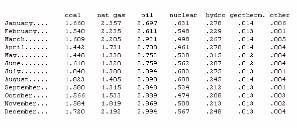
a) Put this data into a format that can be read by MATLAB as 12x7 array and plot(month,energy). You can see some peaks during the winter and the summer. Calculate the average fuel usage per month from all sources, and look at the covariance, producing the covariance matrix. Normalize the elements with the values standard deviation of the i-th and j-th variables. The diagonal elements should thus just become unity, and the off-diagonal elements compare the magnitude of the covariance to the variability of each variable. Where are the strongest positive correlations? Which kind of energy usage shows the largest variability?
b) Calculate numerically the variance in the ratio as a derivatives of the ratio with respect to the variables, and the relative standard deviation.
Exercise 11.
Solve a linear regression problem using QR factorization.
Suppose we want to measure the acceleration due to gravity by measuring the position of a ball as a function of the time after it has been dropped. We know that the position should be given by:
|
where h0 is the initial position and u0 is the initial velocity. Thus if we have the data points (t(i),h(i)) we can fit a parabola to it and get g. We take the data to be given by:
t=[0,.1,.2,.3,.4,.5,.6]' and h=[0.5,14.6,21.0,15.5,2.0,-22.7,-56]'
a) Plot this data: plot(t,h,'o'). The modeling functions are 1,t, and t2, thus the matrix A is given by: n=length(t); a=[ones(n,1),t,t.2]. Solve this using the normal equations: ata=a'*a atb=a'*h and then the solution: x=ata\atb with the gravitational acceleration of: g=-2*x(3). Compare this to the data plotting plot(t,a*x).
b) Do the same thing via QR factorization. First do the QR factorization: [q,r]=qr(a); Note that only upper triangular elements are non- zero. The diagonal elements of this matrix are not necessarily ordered by size, although 'qr' can be set using pivoting to be so. The matrix q is a square matrix with the interesting property that q'*q=eye, that is q is orthogonal. q'*q . We can reduce the problem by multiplying both A and the rhs h by q': qta=q'*a and qtb=q'*h . Note that the last four elements of the new rhs provide the norm of the residual. Solve this: x=r\qtb which gives the same result.
Exercise 12.
Use MATLAB to do a simple error calculation. The example is determining the acceleration due to gravity by measuring the height of a ball as a function of time which is initially thrown upward with some velocity. Set up the array of times: t = [0:.125:2.5]T, and generate some artificial 'data' with random noise: b = 9.8*(1.25t-0.5t2). Add random noise using finction randn.
a) Create the matrix of modelling functions: A = [ones(size(t)),t,t.2]. This is the matrix K used in the solution: K = (ATA)-1AT.
b) Here are the best fit modelling parameters: x = Kb. Estimate the variance in b using MATLAB functions size and norm.
c) Use the variance in b to calculate the variance in x. Generate a smooth curve for the best fit curve: tp=[0:.1:2.5]'; ap=[ones(size(tp)),tp,tp.2]; bp=ap*k*b;
d) Plot this up and calculate the variance in the model predictions.
e) Extract the square root of the diagonal to get the standard deviation, add the 95% confidence interval to the plot, and finish by outputting the best fit parameter values and their standard deviations.
f) Compare the first coefficient with the expected value of 9.8 m/s2.
Exercise 13.
Calculate error in linear regression for a separation process in which the transport of solute molecules is selectively enhanced by oscillating fluid along the length of a pore or a fiber in a membrane. Let's consider the following data for enhancement in the transport of 1-butanol and t-butanol as a function of tidal displacement (the amplitude of oscillation):
tidal=[.0544;.102;.131;.276;.132;.131;.161;.163;.182;.181];
enhancetbut=[.287;1.15;1.45;8.17;1.44;1.58;2.29;2.19;2.88;2.04]*104;
enhance1but=[.407;1.72;2.18;10.06;1.93;2.18;3.17;3.08;4.04;2.66]*104;
a) Display this in matrix form and plot this up using loglog option of plot. As you can see from this plot, we have a power law dependence of the enhancement on the tidal displacement. Also, the enhancement for 1-butanol is greater than that of t-butanol, forming the basis for separation.From theory we expect the enhancement to go as the square of the tidal displacement. We wish to determine if this is satisfied by the data to within error, and to determine the ratio of the enhancements, again with error limits. Do this using linear regression.We expect a power law dependence on tidal displacement, thus we must first convert the model from this non-linear form to a linear form. The modeling parameters are thus the log of the amplitude and the exponent.
b) Solve for the best fit parameters using the normal equations. Calculate the error in the measurements and the error in the slope.
Exercise 1.
The formula for the forward difference algorithm for calculating the derivative of a function is:
|
where h is some small quantity.
Determine the error this formula makes in calculating the derivative of f(x) = ex over the range x Î [0;1], and determine both the minimum error and the optimum value of h. How does this compare to the forward difference formula?
a) Calculate the error for a number of different values of x in order to average out the random round off error. Pick values of h in the range of 10-6 to 10-9. Define h(n) = 10[(-n)/ 10] for n = 60:90. Use the MATLAB function sum to evaluate error. Plot the function error(h) using the MATLAB function loglog
b) Find the value of h, where this function has a minimum. Using a formula for the error of forward differences, evaluate the machine precision.
Exercise2.
a) Use a Taylor series expansion to calculate accurate values near zero for the function
|
b) Determinate limx® 0f(x)
Exercise 3.
The function f(x) is given by
|
a) Write a MATLAB subroutine that computes this function.
b) Plot the function for 1 £ x £ 3, with stepsize 0.01, and print out the plot.
c) Starting with the interval [1;3], how many steps of the bisection method would it take to reduce the interval to the length of less than 10-5?
d) Use Newton's method to find the root to full machine accuracy, starting with x0 = 2. How many iterations does that take?
e) Use the secant method to find the root to full machine accuracy, starting with x0 = 2, x1 = 1.8. How many iterations does that take?
f) Solve the equation for x and ex, and prove, that fixed point iteration will work for x near 2.
g) Find the root to full machine accuracy using the fixed point iteration, starting with x0 = 2. How many iterations does that take?
h) Find the root to full machine accuracy using the MATLAB built-in function fzero . How many iterations does that take?
Exercise 4.
a) Write a MATLAB program using fixed-point iteration to solve
|
b) Prove, that the iteration function converges to the solution.
Exercise 5.
Let
| |||||||||||||||||||||||||||||||||||||||||||||
a) Calculate AB,BA and BTAT, and verify that AB ¹ BA and (AB)T = BTAT.
b) For the 1,2 and ¥ norms, verify that
|
Exercise 6.
Find the condition number of the matrix
| ||||||||||||||
using the infinity-norm.
Exercise 7.
Estimate the condition number of the matrix
| |||||||||||||||||||||||
by solving the linear system Ax = b, with
a) bT = [24,27,27];
b) bT = [24.1,26.9,26.9];
Use iterative improvement.
Exercise 8.
Solve the system
| |||||||||||||||||||||||||
by Jacobi and Gauss-Seidel iterative methods.
Exercise 9.
Find the polynomials of degree 1,2 and 3 which best approximate the following data in the least square sense:
| xi | 0 | 0.15 | 0.31 | 0.5 | 0.6 | 0.75 |
| yi | 1 | 1.004 | 1.031 | 1.117 | 1.223 | 1.422 |
Exercise 10.
Consider the function
|
Use this function to create N data points (N = 4 to 12) in the range x = 0 to 10. Then use the spline function to interpolate at 100 equally spaced points (see command linspace). Compute the exact value of the function at the same interpolation points. To assess the accuracy of the spline interpolation, for each value of N find the maximum absolute error and the RMS error where
|
Plot the maximum error and RMS error versus N and comment on these results.
Exercise 11.
Consider the nonlinear system of equations
|
Find a solution near x0 = (0.1;0.3)T.
a) Write a MATLAB subroutine to evaluate f(x) and its derivative Df(x) (which is a 2x2 matrix). Print out f(x0) and Df(x0).
b) Do four steps of Newton's method on the problem. That shoud give you the answer to full machine accuracy.
c) Use the MATLAB built-in function fsolve. The default accuracy is 10-4. How many iteration steps does it take?
Exercise 12.
The two functions represent a parabola and an ellipse, respectively
|
Write a program to implement the Gauss-Seidel iteration method with relaxation to solve this system and find the intersection coordinates to the 4th significant digit. Experiment with the program to determine the effects of different formulations, first guesses, and relaxation. Summarize your experimental results in a concise (hand-written is acceptable) summary table. Have you been able to locate both solutions? Comment on the results in the table and make a list of the advantages and disadvantages of this method.
Exercise 13.
Numerically solve the equation x¢ = x(1-x) with x(0) = .01 with 0 < t < 5 and plot the solution (x¢ means dx/dt in this context).
Use [t z] = ode23('myfun',t0,tf,z0) where you have a separate file called 'myfun.m defined as function myfun=myfun(t,z).
Exercise 14.
a) Consider the differential equation y¢¢+ty = 0 , y(0) = 0 , y¢(0) = 1. Find the values of y¢¢(0),y¢¢¢(0) and y¢¢¢¢(0).
b) Use the values of the derivatives of y(t) to construct a Taylor polynomial approximation to the solution y(t). Plot and print graphs of y(t), the Taylor polynomial approximation, and the difference between y(t) the Taylor polynomial over the interval [0;10]. Use ode23 or ode45 to help plot the ``exact'' solution.
c) For which values of t is the Taylor polynomial a qualitatively good approximation to y(t)? Is this what you would expect? What degree polynomial would you need to get a ``good'' approximation across the whole interval [0;10] ?
Exercise 15.
a) Find the general solution to the system x¢ = Ax, where
| |||||||||||||||||||||||||||||||||||||||||||||||||||||
b) Find the solution to the system with initial conditions x(0) = x0, where
| |||||||||||||
Exercise 16.
Solve the harmonic oscillator problem
| ||||||||||||||||||||||||||||
by Runge-Kutta Method.
Use ode45 and plot (y1,y2),(t,y1) and (t,y2), when t0 = 0 and T = 4p with t = linspace(t0,T,300).
Exercise 17.
Find the following integral
|
using Simpson 1/3 rule and the MATLAB function trapz. Prepare a table of results containing data that illustrates the effect of step size on accuracy and flop count. Discuss these results.
Exercise 18.
Consider the initial value problem given by the first order ODE
|
along with the initial condition y = 0 at t = 0.
Write two MATLAB functions to solve this ODE using Euler's method and the 4th order RK, respectively. Try to generalize your code so that the functions are called as follows: [t, y] = euler('function',a,b,y0,h) and [t, y] = rk4('function',a,b,y0,h) where function is the name of an out-board MATLAB function to evaluate f(t,y) defined by the ODE: [dy/ dt] = f(t,y). The arguments a and b are the initial and final values of t, y0 is the initial condition, and h is the constant solution stepsize. A single call to this function should result in the two vectors t and y being returned containing the solution data.
Solve the given ODE for the interval from t = 0 to t = 10. You might like to plot the exact solution as a solid line and the numerically computed solution values as symbols. For stepsizes ranging from h = 1 down to h = 0.005 determine the maximum error that occurs over the solution range (this may not be at t = 5 but might occur earlier). Also for each stepsize chosen, determine the flopcount for the solution.
Plot the following graphs showing data for both solution methods on each graph:
1.Maximum error versus stepsize
2.Maximum error versus flopcount
You might consider using a loglog plot for these graphs. Comment on these results.
WebMaster AK
