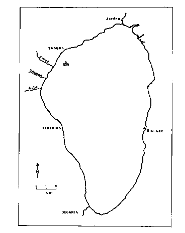
 Fig. 1. Lake Kinneret, stations where the wind was measured: A BB-Tabgha; 0 -Ein-Gev.
(Accepted for publication 6 August 1982)
Abstract
H. Volohonsky, A. Kaplunovsky, and S. Serruya, 1983. Storms on Lake Kinneret: observations and mathematical model Ecol. Modelling, 18: 141-153, (1983)
The descriptive model, which builds typical storm-still patterns on a monthly basis, is discussed. Storms formed by the model are events having three measurable parameters: time of start, duration and mean wind speed. The model considers the interrelations between these parameters. The model output is designed to be used in the ecological model.
INTRODUCTION
The significance of storms for the Lake Kinneret ecosystem and the way these events are formed from hourly measurements of the wind speed have already been discussed in our former publication (Volohonsky et al., 1980), which contains the basic principles of "event-oriented approach" to modelling of thermal stratification, appropriate references, and description of what we call "storms" and "stills", the latter briefly repeated here.
The submodel SELWD chooses from hourly measurements a consecutive set D (D>Dk = 4 h) of hourly values of wind speed Wi≥Wk = 6 m s-1. This period is called " the storm", with duration of D hours and wind speed W equal to the arithmetic mean of Wi.
The third parameter of the storm is its starting time B, hours a.m., defined in the same submodel. The intervals between two storms are specified as 6 6 stills" and the wind speed of the still is calculated in the same way as for storms. In such a way, information about the wind pattern is chunked and the astronomic time scale is replaced by the time scale of "events", i.e. 6 6 storms" and "stills", in order to be used in other submodels pertaining to the general ecological model of Lake Kinneret (GEMLK).
The work of SELWD with the set of observations during the period 1970-77 recorded by S. Serruya (at Tabgha Station, Fig. 1) gave about 1500 stormy events. In this paper we present the statistical analysis of storm parameters on a time scale of one year and we describe the mathematical model MONSTR which builds storm patterns for each month.
 Fig. 1. Lake Kinneret, stations where the wind was measured: A BB-Tabgha; 0 -Ein-Gev.
Distribution of storms on a year time scale
The storms obtained as an output of SELWD from wind speed measurements we shall call here "observed" storms. The number of storms in different months throughout the period of observation varied from 33 (February) to 247 (July). These numbers are high enough for statistical analysis. The mean number of storms per each month could not be calculated directly, since the set of measurements for Tabgha station was not absolutely continuous. It, as well as the limits, was roughly estimated using some data from Ein-Gev station. The numbers of storms that qualified as 66average", "high" or "low" are displayed in Table 1.
TABLE I

Number of storms per month for three typical regimes (H - high number of storms; A - average; L - low)

________________________________________________________________________________________
 Month          I    II    III   IV     V    VI   VII   VIII   IX     X    XI    XII
________________________________________________________________________________________

          H    13    11    14    20    28    29    30    30    28    13     9    12
 Regimes  A     9     6     9    13    23    28    30    30    23    11     6     8
          L     5     2     4     5    18    25    30    30    20     7     3     4
________________________________________________________________________________________
Characteristics of the total set of observed storms
The characteristic of the event which we call "storm" is built up of three formally independent but not necessarily physically independent parameters: the time when it starts (B, hours) its duration (D, hours) and its average wind speed (W, m s-1). According to the accepted formalism, the values of B and D are integers, W has one decimal after the point. The mean values and standard deviations of these parameters for the whole set of 1464 storms from Tabgha station are presented in Table II.
TABLE II

Averaged characteristics of a storm on Lake Kinneret


	Parameter	Mean	S.D.	Limits:
				mean + 1 S.D.

	B, h (a.m.)	12.7	2.9	10.00-16.00 a.m.
	D, h		7.8	4.2	4 -12 h
	W, m s-1		8.8	1.2	7.6 -10.0 m s-1
The results of the preliminary analysis may be summarized as follows: 67% of the storms start between 10.00 and 16.00, have a duration of 4-12 h and an average wind speed of 7.6-10.0 m s-1. The most stable characteristic is the time when the storm starts (B). The histograms presented in Fig. 2 are "hump-like" and show marked asymmetry especially for the storm duration. The multiple regression analysis has shown that all three parameters are correlated significantly for 0.995-level (Table III). The equations give evidence that (a) the storms which start earlier are longer; (b) the duration of weaker storms is longer-the latter interrelation (b) being less pronounced than the former (a).
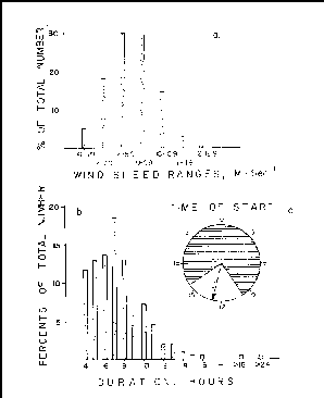 Fig. 2.
Parameters of storms (Tabgha, the total set), (a) histograms of wind speeds W, (b)
histograms of durations (D), (c) starting time (B). White sector represents the limits,
specified by 1 S.D. The arrow points to the hour when the maximum of storms start and the
figure above the arrow indicates the number of these storms in % of total.
Characteristics of storms for specific months
We have performed similar statistical analysis of SELWD output for each month throughout the whole set of observations. The mean values and standard deviations of storm parameters are displayed in Table IV, the histograms in Figs. 3, 4 and 5. We could not find any regular function to approximate the observed distributions. The differences between the distributions of two consecutive months appeared to be significant (0.95 level, Kolmogorov-Smirnov two sample test, in Campbell, 1967: pp. 56-57), at least for one of the storm parameters, in all the cases except December-January and March-April; it demonstrates the high specifity of monthly storm patterns. Wind speed is the most informative parameter, the starting time and duration are, in general, less specific.
TABLE III

Multiple regression equations for the total set of storms on Lake Kinneret


No.	Equation		   Standard   Dimension   Correlation   F-statistic
				   error		  coefficient


I	D= 26.6	- 0.888 x B	    5.36	 h	   0.590	  702
		- 0.839 x W						  53.4
2	W= 9.50 - 0.0315 x B       1.21          m s-1      0.191	  11.7
		- 0.0429 x D					          53.4
TABLE IV

Parameters of storms (means and standard deviations) for each month. The vertical bar between two adjacent values means that
distributions of appropriate parameters differ significantly for 0.95-level, Kolmogorov-Smirnov two-sample test


Month	XII	I	II	III	IV	V	VI	VII	VIII	IX	X	XI	XII

No. of	37	46	33	56	90	160	221	247	241	185	88	44	37
storms
B	8.25	10.2	8.98	11.9	12.2	13.0	12.7	12.3	12.8	13.4	13.6	12.4	8.25
S.D.	6.01	6.18	5.57	4.09	3.17	2.25	1.97	1.81	1.63	1.29	2.87	5.92	6.01
D	13.5	11.3	12.5	6.84	7.27	6.79	7.94	8.55	7.70	6.36	5.93	9.84	13.5
S.D.	10.2	9.47	12.6	3.46	3.04	2.09	2.47	2.33	1.98	1.69	2.26	7.22	10.2
w	7.84	7.45	8.14	8.16	8.39	8.69	9.13	9.58	9.37	8.78	8.07	7.58	7.84
S.D.	1.02	0.80	1.22	0.86	0.96	1.00	1.08	1.01	1.03	0.98	0.89	0.66	1.02
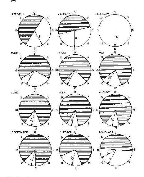 Fig. 3.
Starting time (on monthly basis). See comment to Fig. 2c.
The multiple regression analysis has shown the absence of correlations significant for 0.995-level between any combination of storm parameters in December, January, February and March. The regression equations for the rest of the months are shown in Table V. The form of equations fo April-October with higher correlation coefficients and F-statistics (eqs. 1, 2, 3, 4, 7, 9 and 13, Table V) is in qualitative agreement with the evidence obtained from the whole set that the storms which start earlier last longer The feature of the whole set, that the longer storms are weaker, has been observed in June, July, September and November (eqs. 4, 6, 8, 12 and 14, Table V). But only three equations (4, 6 and 12, Table V) from the monthly sets appeared to have the same shape as those for the total set (eqs. I and 2, Table III), a fact confirming the high specificity of monthly storm patterns.
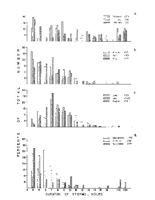 Fig. 4.
Monthly histograms of storm duration (a - winter; b - spring; c - summer;
d - autumn).
TABLE V


Multiple regression equations of storm parameters for each month, significant for 0.995-level


Month	No.	Equation			Standard	Dimension	Correlation		F-statistic	Comment
						error				coefficient R


IV	1	D =	11.2	- 0.317 x B	2.99		h		0.331			10.9		used
V	2	D =	14.6	- 0.598 x B	1.56		h		0.650			114		used
VI	3	D =	17.9	- 0.779 x B	2.03		h		0.624			134		used
	4	D =	24.6	- 0.872 x B	1.92		h		0.675			172		not used
				- 0.610 x W								25.4
	5	W =	11.0	- 0.152 x B	1.10		m s-1		0.277			17.4		not used
	6	W =	14.1	- 0.291 x B	1.04		m s-1		0.420			43.5		used
				- 0.178 x D								25.4
VII	7	D =	19.2	- 0.871 x B	1.79		h		0.671			188		used
	8	W =	8.75	- 0.0855x D	0.978		m s-1		0.206			10.2		rejected a priori
VIII	9	D =	20.1	- 0.973 x B	1.20		h		0.801			422		used
IX	10	D =	15.0	- 0.962 x W	3.14		h		0.357			26.9		not used
	11	W =	14.9	- 0.457 x B	1.04		m s-1		0.551			80.3		not used
	12	W =	15.2	- 0.426 x B	0.979		m s-1		0.622			77.5		used
				- 0.108 x D								24.9
X	13	D =	9.61	- 0.297 x B	2.80		h		0.428			17.9		used
XI	14	D =	63.0	- 6.94  x W	8.73		h		0.664			34.7		used
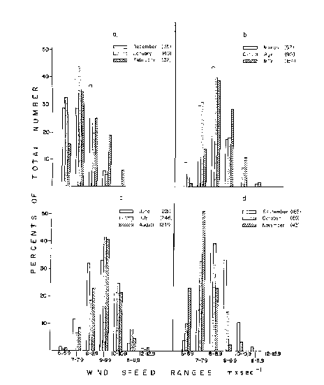 Fig. 5.
Monthly histograms of storm wind speed (a - winter; b - spring; c - summer;
d - autumn).
Physical background
The observed drastic difference between the storms of the winter period and those of the rest of the year may be related to their different origin. According to Neuman and Stanhill (1978) the summer storms on Lake Kinneret are, in essence, Mediterranean breezes amplified over the lake. Thus, the breeze speed being about 5 m s-1 at the Mediterranean shore may reach more than 10 m s-1 at the lake due to rift relief (catabatic winds). These western storms occur nearly every day in June, July and August, and less regularly in April, May, September and October, and constitute 83% of the total observed numbers. The storms occurring during the rest of the year originate from meteorological situations of different scales and their characteristics are less uniform. The total set of observed storms is actually built up of two distinct sets: "catabatic winds" and "other storms". The regression equations of Table V seem to describe the properties of the storms of the first type (except eq. 14, for November).
Stills
The B and D parameters of stills are strictly defined by the corresponding parameters of storms. The only free parameter of stills is the mean wind speed W, which is equal to 2.67 m s-1 and S.D. = 0.61 m s-1 for the total set, twice as small as the standard deviation of the same parameter of storms-the wind speed of stills being more stable. The distribution is slightly asymmetric: the mode value is 2.60 m s-1 , practically equal to the median. The differences between two consecutive months appeared to be negligible. Winter stills (December-February) in total had an averaged wind speed value of 2.88 m s-1 , slightly higher than the stills of the rest of the year (2.65 m s-1 This feature has been ignored in the model.
MODELLING
Description
The information concerning "storms" and "stills" parameters has been used in a very simple, descriptive (iion-explanatory) model, MONSTR, which builds specific storm-still patterns for the period of one month.
The role of MONSTR in a structure of GEMLK is clear from Fig. 6, its working cycle is presented in Fig. 7. In certain cases we wish not to be dependent on the field data, in order to be able to investigate ultimate situations which are not always represented in a restricted set of observations. Then, instead of an observed set of SELWD output used for the calibration of our WBIOTOP model (mixing between epi-, meta- and hypolimnion), we work with MONSTR output.
The number of storms for a definite month may be given arbitrarily, but as a rule is taken from Table I, corresponding to one of three typical regimes. The date of a storm is chosen randomly, but should be corrected if two storms overlap or if a still between them appears to be shorter than 4 hours; the B-parameter is chosen at random from frequency histograms of each month; D and W parameters are also chosen at random from the histogram if they are not inter-correlated significantly with B. In the latter case, one of the regression equations from Table V (as a rule, the one which has the highest significance level) may be used with certain precautions: the equation which markedly influences the mean value or frequency histogram, or cuts off an important range of values should be rejected a priori. The value of a parameter calculated from the regression equation is randomized in limits specified by the standard error.
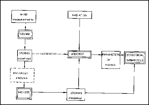 Fig. 6.
The place of MONSTR in the structure of the general ecological model.
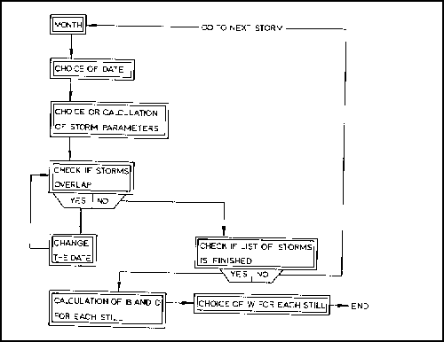 Fig. 7.
Working cycle of MONSTR.
Validation
This procedure is simply a comparison of the frequency histograms (X2-criterion) of a-certain parameter obtained as MONSTR output (three model runs with three typical regimes of Table 1) with those of the observed set provided by SELWD output. The significance level has been chosen as 0.975 for X2-test (with not less than 3 degrees of freedom, i.e. 4 ranks). If the calculated criterion appears to be higher than that specified by the signifi- cance level, then the null hypothesis: "MONSTR output is identical to SELWD output" is to be rejected as well as the corresponding regression equation. The valid equations are indicated in Table VI, and X2-criteria for monthly sets of parameters calculated from these equations are in the same table.
TABLE VI

Validation of MONSTR output


	Month	Equation No.	Degrees		X2-test		Decision
		(from Table V)	of freedom

	IV	1		9		13.00		Valid
	V	2		8		15.22		Valid
	VI	3		10		16.05		Valid
		6		6		33.52
				3		8.74		Valid
	VII	7		10		13.66		Valid
	VIII	9		10		25.82
				5		5.27		Valid
	IX	12		5		3.70		Valid
	X	13		5		18.69
				3		12.87		Invalid
	XI	14		4		7.19		Valid
DISCUSSION
Equation 13, for October, gave invalid output when used in MONSTR. The reason may probably be of a physical nature: October is a month when the Mediterranean breezes are not formed regularly enough, the observed set being actually a mixture of events with different time and space scales, and the regression equation, though significant as such, fails to express certain features of the distribution of storm parameters. In this case we neglect the correlation between the parameters and choose all of them from frequency histograms.
CONCLUSIONS
The presented matter is an example of an event-oriented approach to ecological modelling. The "storms" are not pure results of direct measure- ments but entities formed by a more complex procedure, which includes an epistemological effort. Though losing some information, we thereby gain clearness and simplicity. The "events" may be modelled easily, and the interpretation of results poses no problem since the language of the model is rather close to the non-formal human language. The durations of stills and storms provide one of the basic time-scales for other submodels of GEMLK.
REFERENCES
WebMaster AK
